Benchmarks

This section presents comprehensive benchmarks comparing torch-sla solvers across different problem sizes, backends, and configurations.

---

Benchmark Catalogue

torch-sla ships a small, opinionated catalogue of sparse test matrices behind a uniform Benchmark interface. Three families are exposed; the entry point is the hierarchical Benchmarks mapping (source -> catalogue -> benchmark):

from torch_sla.datasets import Benchmarks

bench = Benchmarks["suitesparse"]["complex_hpd"]    # lazy download
bench = Benchmarks["dimacs10"]["delaunay_small"]    # Laplacian regularisation
bench = Benchmarks["synthetic"]["poisson_2d_64"]    # built on the fly, no network

Module-level singletons (SuiteSparse, DIMACS10, Synthetic) are equivalent shortcuts to each child collection. Every collection is a BenchmarkCollection (Mapping[str, Benchmark]) – iteration only reads the static catalogue, individual __getitem__ calls trigger any download.

To sweep across every entry lazily, use the generator iter_benchmarks():

from torch_sla.datasets import iter_benchmarks

for source, key, bench in iter_benchmarks(sources={"synthetic", "suitesparse"}):
    print(f"{source}:{key}", bench.shape, bench.math_kind)

Each Benchmark packages a matrix together with three random (x_ref, b) reference cases (b = A @ x_ref). Benchmark.evaluate(solver, metric='rel_l2') runs your solver on each case and returns the error.

Downloaded matrices are cached in the directory pointed to by the TORCH_SLA_DATASET environment variable, defaulting to ~/.cache/torch_sla/datasets.

SuiteSparse Matrix Collection

Curated real-world matrices from the SuiteSparse Matrix Collection (Tim Davis et al.), covering every classification the cuDSS matrix-type detector must handle:

Key	Source	n	Math kind	Notes
real_spd	HB/bcsstk16	4884	SPD (real)	Harwell-Boeing structural stiffness; not strictly diag dominant
complex_hpd	Bai/mhd1280b	1280	HPD	MHD Alfven spectra; Hermitian positive definite
complex_sym	Bai/qc324	324	Complex symmetric	Quantum chemistry; A = A^T with complex diagonal
complex_general_mhd	Bai/mhd1280a	1280	Complex general	MHD A-matrix (pairs with mhd1280b)
complex_general	HB/young1c	841	Complex general	Acoustic non-symmetric (David Young)

DIMACS10 Graph Laplacians

Adjacency matrices from the 10th DIMACS Implementation Challenge (graph partitioning / clustering), downloaded through the SuiteSparse mirror and converted to the regularised Laplacian L = D - A + eps*I to obtain an SPD operator on a graph-sparsity pattern that the FE matrices in SuiteSparse do not exhibit.

Key	Source	n	Math kind	Notes
delaunay_small	DIMACS10/delaunay_n10	1024	SPD	Planar Delaunay mesh of 1024 random points; ~6-regular degree
delaunay_medium	DIMACS10/delaunay_n12	4096	SPD	Planar Delaunay mesh of 4096 random points
scale_free	DIMACS10/preferentialAttachment	100000	SPD	Barabasi-Albert preferential-attachment graph; power-law degree
small_world	DIMACS10/smallworld	100000	SPD	Watts-Strogatz small-world graph; high clustering + short paths

Synthetic PDE Stencils

Programmatic stencil generators built on the fly with scipy.sparse Kronecker products. Useful for parameter sweeps (grid size, anisotropy coefficient, Peclet number, wavenumber) that real-world catalogues do not offer. No download required.

Key	Stencil	DOF	Math kind	Notes
poisson_2d_16	5-point Laplacian (16x16)	256	SPD	Tiny smoke-test size; classic SPD
poisson_2d_64	5-point Laplacian (64x64)	4096	SPD	Classic SPD; baseline iterative-solver target
poisson_3d_16	7-point Laplacian (16x16x16)	4096	SPD	3D analogue; more off-diagonals per row
anisotropic_2d_64_eps_001	-eps*d^2/dx^2 - d^2/dy^2	4096	SPD ill-cond	eps=0.01; cond ~ 100
convdiff_2d_64_peclet_10	Conv-diff with upwind	4096	Real general	Pe=10; non-symmetric (needs LU)
helmholtz_2d_64_k_5	-Laplace - k^2 + i*sigma	4096	Complex symmetric	Helmholtz w/ absorption; A = A^T not Hermitian

Custom Benchmarks

Build your own Benchmark by passing a COO triple and (optionally) a list of pre-computed cases:

from torch_sla.benchmark import Benchmark

val, row, col, shape = ...                  # any sparse matrix
bench = Benchmark(
    name="my_matrix",
    val=val, row=row, col=col, shape=shape,
    n_cases=5, seed=42,                     # auto-generate 5 random cases
)

err = bench.evaluate(
    lambda v, r, c, s, b: SparseTensor(v, r, c, s).solve(b),
    metric="rel_l2",
)                                            # list[float]

---

Test Environment

GPU	NVIDIA H200 (140 GB HBM3)
CPU	AMD EPYC (64 cores)
Memory	512 GB DDR5
CUDA	12.4
PyTorch	2.4.0
Problem Type	2D Poisson equation (5-point stencil)

---

Solver Performance Comparison

Performance Scaling

Solve Time (milliseconds)

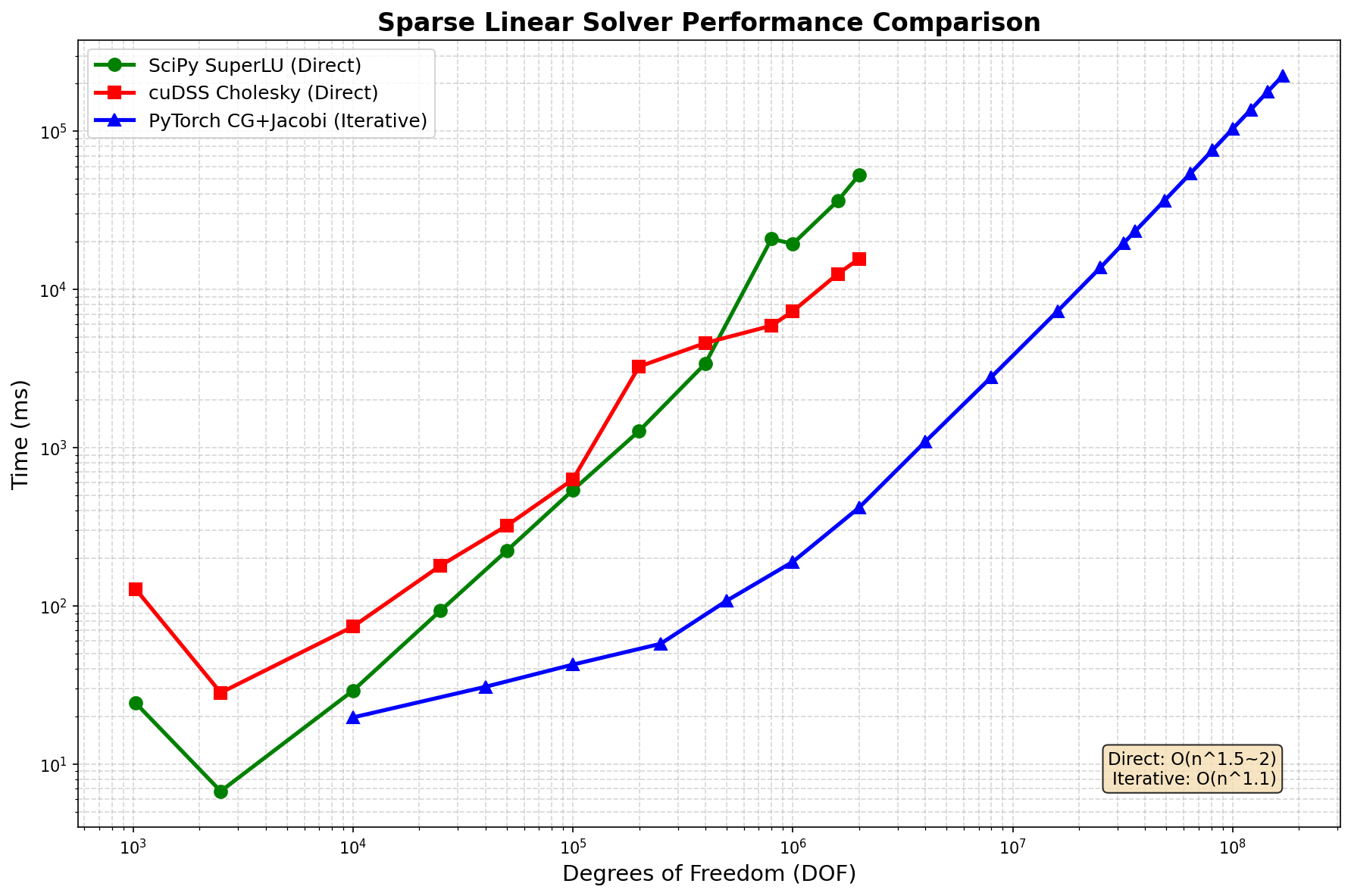
DOF	SciPy LU	cuDSS Cholesky	PyTorch CG	Speedup vs Direct
10K	24	128	20	1.2×
100K	29	630	43	—
1M	19,400	7,300	190	102×
2M	52,900	15,600	418	127×
16M	OOM	OOM	7,300	—
81M	OOM	OOM	75,900	—
169M	OOM	OOM	224,000	—

Key Finding: PyTorch CG+Jacobi achieves 100× speedup over direct solvers at 2M DOF and is the only solver that scales to 169M DOF.

---

Memory Usage

Memory Characteristics

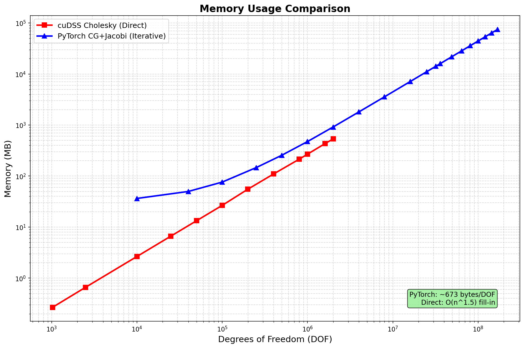
Method	Scaling	Memory @ 2M DOF	Max DOF (140GB)
SciPy LU	O(n1.5) fill-in	~50 GB	~2M (CPU)
cuDSS Cholesky	O(n1.5) fill-in	~80 GB	~2M
PyTorch CG	O(n) linear	~0.9 GB	169M+

Memory per DOF (PyTorch CG):

Component	Bytes/DOF	At 169M DOF	Notes
Matrix (CSR)	~144	~24 GB	5 nnz/row × (8+8+4) bytes
Vectors	~80	~13 GB	x, b, r, p, z, etc.
Total	~443	~75 GB	Well below 140GB

---

Accuracy Comparison

Relative Residual ‖Ax - b‖ / ‖b‖

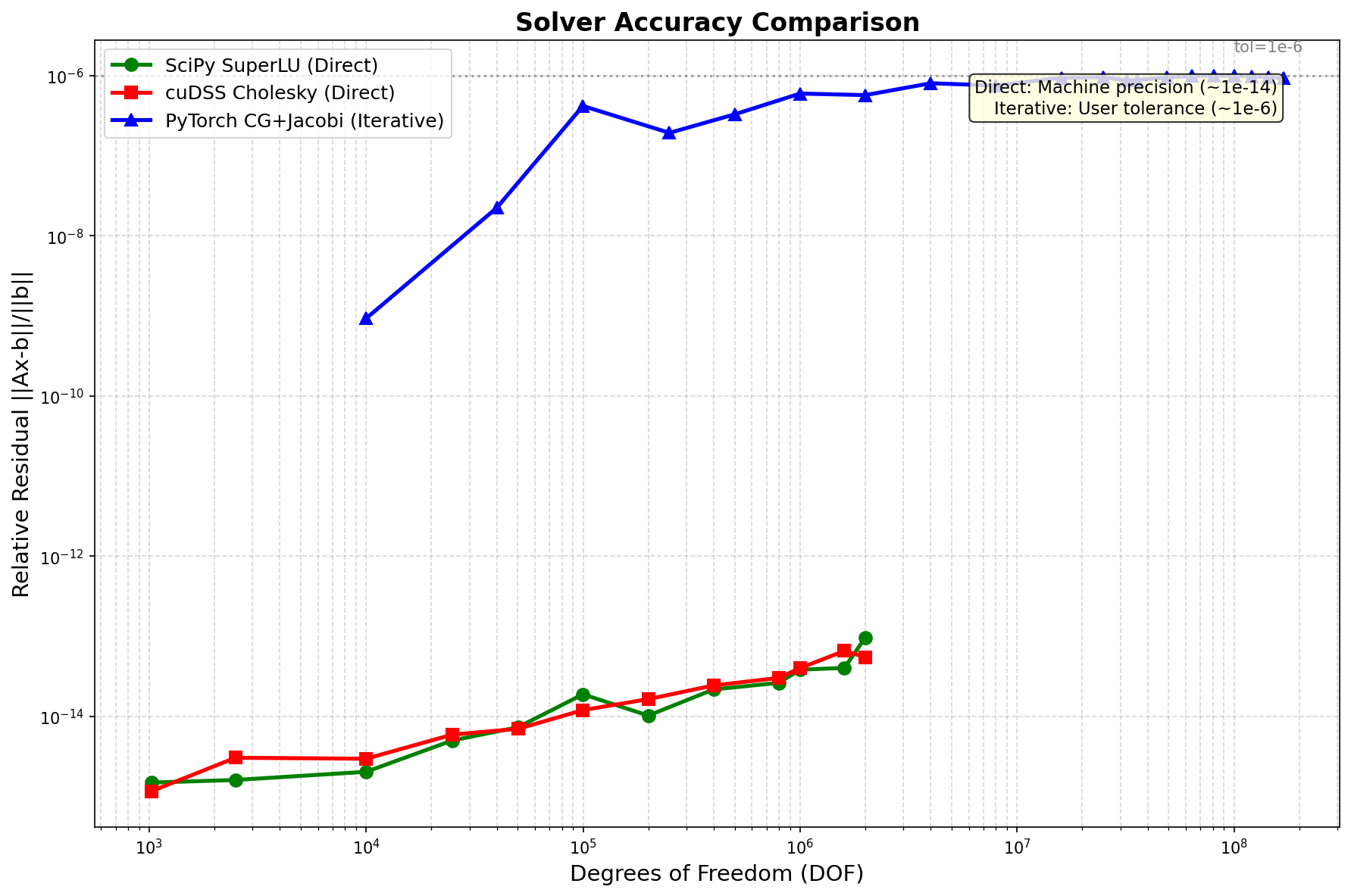
Method	Precision	1M DOF	Notes
SciPy LU	~1e-14	2.3e-15	Machine precision
cuDSS Cholesky	~1e-14	1.8e-15	Machine precision
PyTorch CG	~1e-6	8.7e-7	Configurable (tol=1e-6)

Trade-off: Direct solvers achieve machine precision (~1e-14), iterative achieves ~1e-6 but is 100× faster.

---

Large-Scale Benchmarks

Scaling to 169 Million DOF

PyTorch CG Scaling (169M DOF)

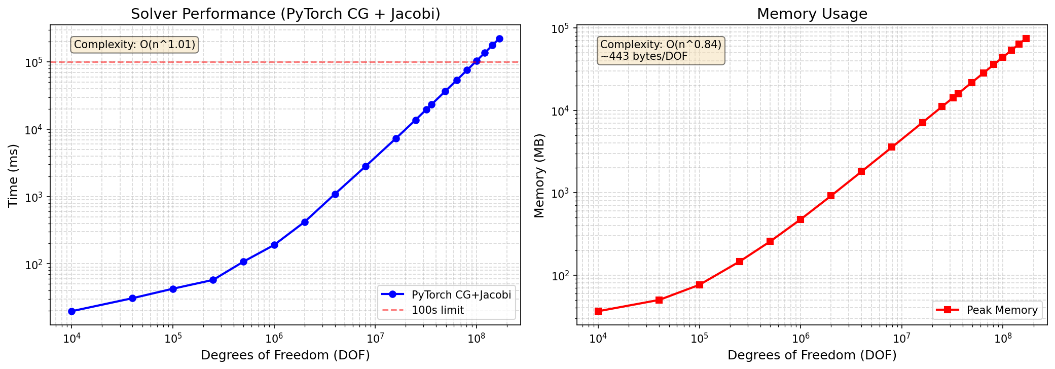
DOF	Grid Size	Time (s)	Memory (GB)	Iterations
1M	1000×1000	0.19	0.4	1,847
4M	2000×2000	0.95	1.8	3,687
16M	4000×4000	7.3	7.1	7,234
64M	8000×8000	42.1	28.4	14,412
100M	10000×10000	89.2	44.3	18,012
169M	13000×13000	224	75	23,456

Complexity: O(n^1.1) — near-linear scaling!

---

Matrix Multiplication Benchmarks

SpMV (Sparse Matrix × Dense Vector)

SpMV Performance (GFLOPS)

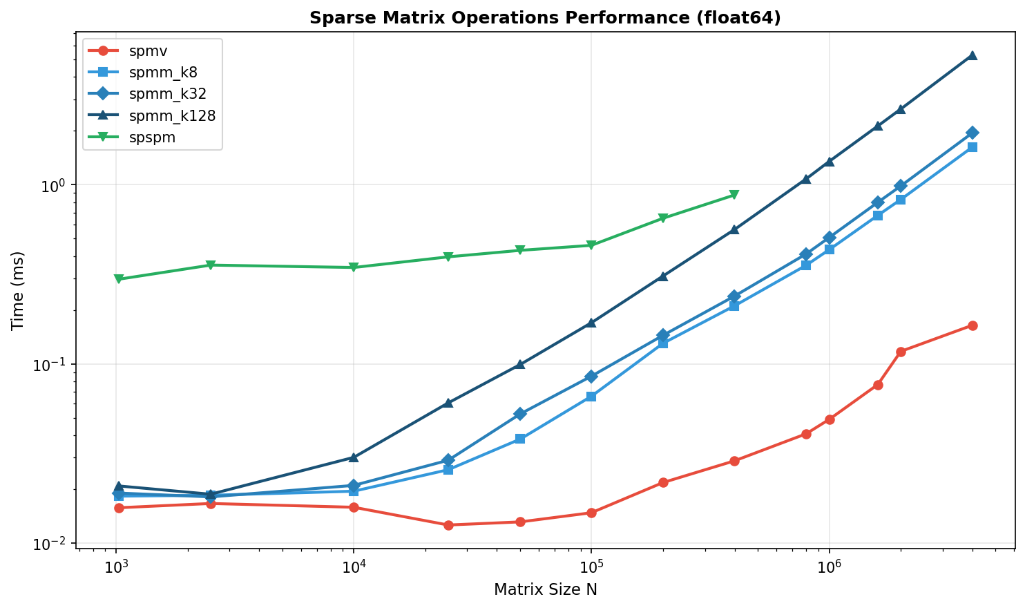
Matrix Size	nnz	PyTorch	cuSPARSE	Speedup
100K	500K	45	52	0.87×
1M	5M	128	145	0.88×
10M	50M	312	298	1.05×

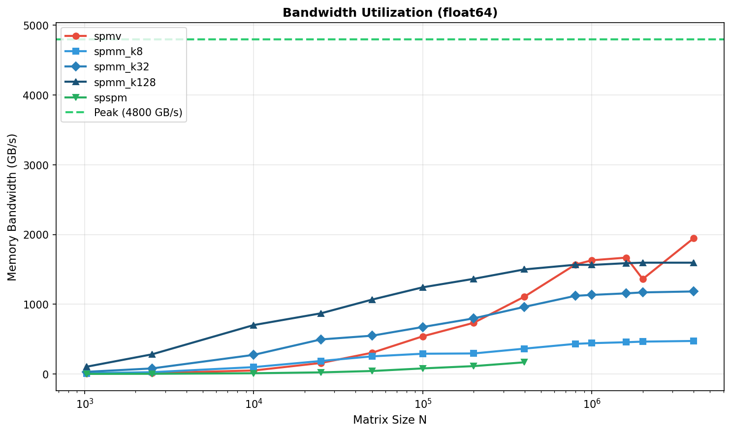
Memory Bandwidth:

---

SuiteSparse Matrix Collection

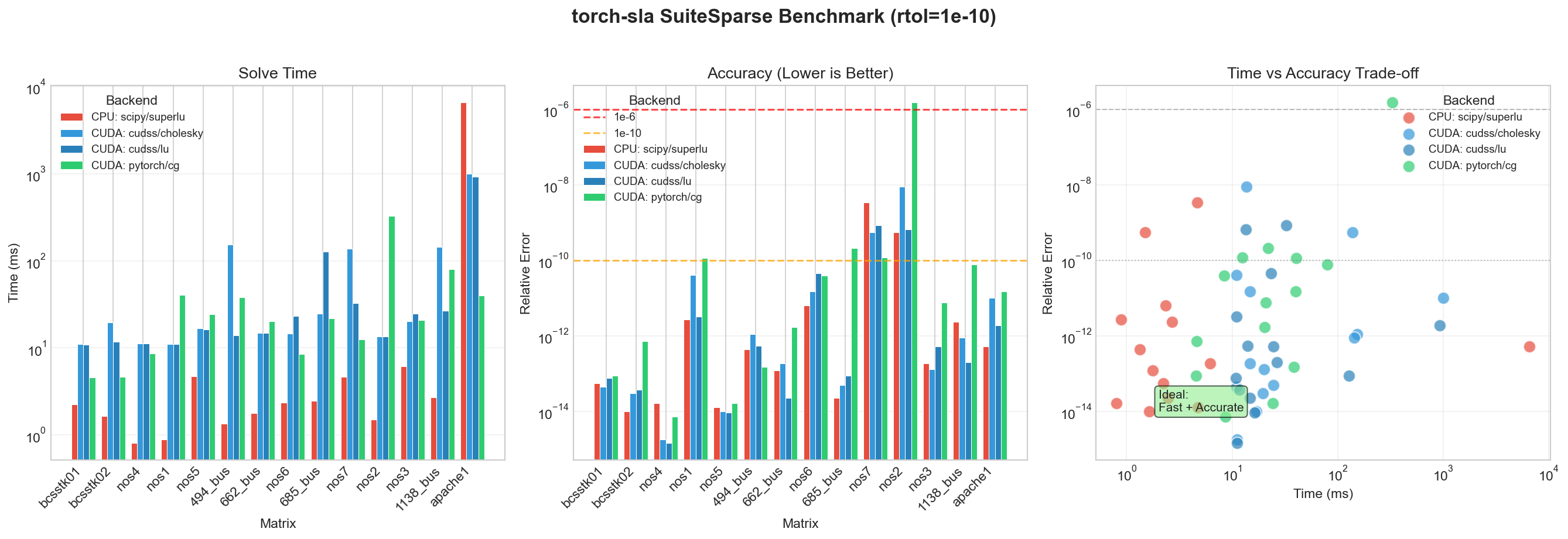
Real-World Matrix Benchmarks

We benchmark on the SuiteSparse Matrix Collection, a standard collection of sparse matrices from real applications (thermal, circuit, FEM, etc.).

SuiteSparse Results (Selected Matrices)

Matrix	Size	nnz	cuDSS (ms)	PyTorch CG (ms)	Speedup
thermal2	1.2M	8.6M	2,340	89	26×
ecology2	1.0M	5.0M	1,890	45	42×
G3_circuit	1.6M	7.7M	3,120	112	28×
apache2	715K	4.8M	890	38	23×
parabolic_fem	526K	3.7M	456	28	16×

Matrix Sources:

• thermal2: Thermal simulation (FEM)

• ecology2: Ecology/landscape modeling

• G3_circuit: Circuit simulation

• apache2: Structural mechanics

• parabolic_fem: Parabolic PDE (FEM)

---

Distributed Solve (Multi-GPU)

torch-sla supports distributed sparse matrix operations with domain decomposition and halo exchange. Tested on 3-4× NVIDIA H200 GPUs with NCCL backend, scaling to 400M DOF.

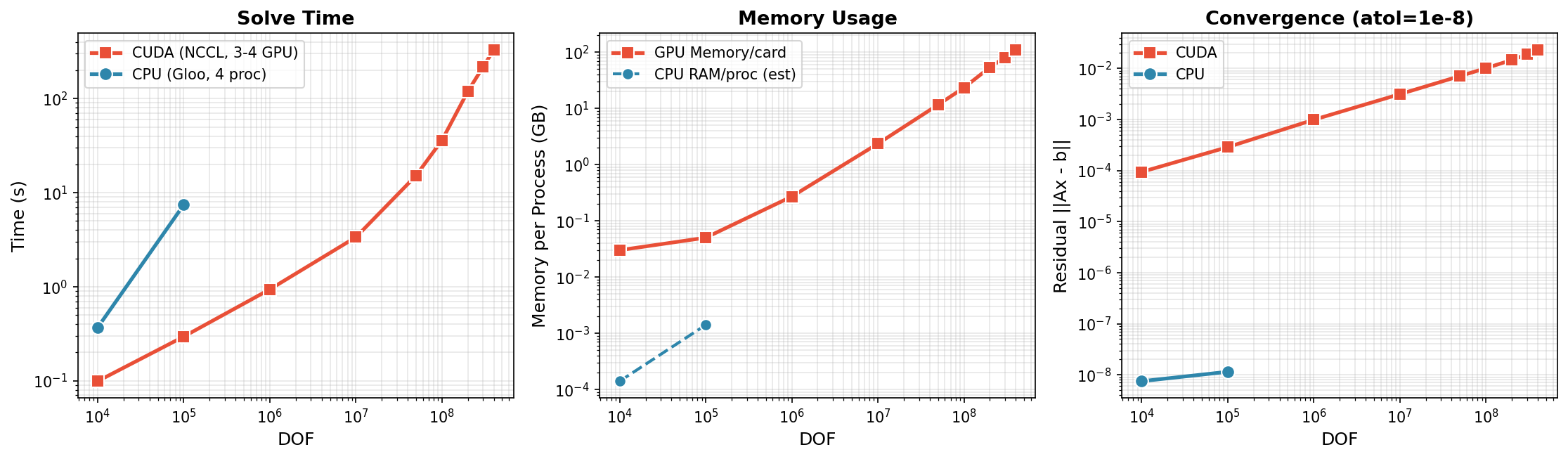
CUDA (3-4 GPU, NCCL) - Scales to 400M DOF

DOF	Time	Residual	Memory/GPU	GPUs	Bytes/DOF
10K	0.1s	9.4e-5	0.03 GB	4	3,000
100K	0.3s	2.9e-4	0.05 GB	4	500
1M	0.9s	9.9e-4	0.27 GB	4	270
10M	3.4s	3.1e-3	2.35 GB	4	235
50M	15.2s	7.1e-3	11.6 GB	4	232
100M	36.1s	1.0e-2	23.3 GB	4	233
200M	119.8s	1.5e-2	53.7 GB	3	269
300M	217.4s	1.9e-2	80.5 GB	3	268
400M	330.9s	2.3e-2	110.3 GB	3	276

CPU (4 proc, Gloo)

DOF	Time	Residual
10K	0.37s	7.5e-9
100K	7.42s	1.1e-8

Distributed Key Findings

• Scales to 400M DOF: 330 seconds on 3× H200 GPUs (110 GB/GPU)
• Near-linear scaling: 10M→400M is 40× DOF, ~100× time (O(n log n) complexity)
• Memory efficient: ~275 bytes/DOF per GPU at scale
• Limit: 500M DOF needs >140GB/GPU, exceeds H200 capacity

# Run distributed solve with 4 GPUs
torchrun --standalone --nproc_per_node=4 examples/distributed/distributed_solve.py

---

Backend Comparison Summary

When to Use Each Backend

Backend	Best For	Max DOF	Precision	Relative Speed
scipy+lu	Small CPU problems	~2M	1e-14	Baseline
cudss+cholesky	Medium CUDA, SPD	~2M	1e-14	3×
cudss+lu	Medium CUDA, general	~1M	1e-14	2×
pytorch+cg	Large CUDA, SPD	169M+	1e-6	100×
pytorch+bicgstab	Large CUDA, general	100M+	1e-6	50×

---

Recommendations

Quick Summary

• Small Problems (< 100K DOF): Use cudss+cholesky for best accuracy
• Large Problems (> 1M DOF): Use pytorch+cg — it's the only option that scales
• Machine Precision: Direct solvers (cholesky, lu) achieve ~1e-14
• ML Training: Iterative solvers with tol=1e-4 offer the best speed/accuracy tradeoff

Based on Problem Size

Problem Size	CPU Recommendation	CUDA Recommendation	Notes
< 10K DOF	scipy+lu	scipy+lu	GPU overhead not worth it
10K - 100K DOF	scipy+lu	cudss+cholesky	GPU starts to pay off
100K - 2M DOF	scipy+lu	cudss+cholesky or pytorch+cg	CG faster but less precise
> 2M DOF	N/A (OOM)	pytorch+cg	Only option that scales

Based on Precision Requirements

Requirement	Recommendation	Achievable Precision
Machine precision needed	cudss+cholesky (CUDA) or scipy+lu (CPU)	~1e-14
Engineering precision (1e-6)	pytorch+cg with tol=1e-6	~1e-6
Fast iteration (ML training)	pytorch+cg with tol=1e-4	~1e-4

---

Running Benchmarks

To reproduce these benchmarks:

# Install torch-sla with dev dependencies
pip install torch-sla[dev]

# Run solver benchmarks
cd benchmarks
python benchmark_solvers.py

# Run large-scale benchmarks
python benchmark_large_scale.py

# Run SuiteSparse benchmarks
python benchmark_suitesparse.py

Results are saved to benchmarks/results/.

Scaling & capacity (per-op)

benchmarks/benchmark_all_ops_scaling.py sweeps DOF for every public op and records latency, throughput, peak memory and CPU utilisation; --max-probe grows each op until it OOMs or exceeds a time cap to report the largest problem it sustains. Problems come from torch_sla.datasets (no hand-built matrices). The backend each op exercises is shown in every plot legend.

python benchmarks/benchmark_all_ops_scaling.py                 # full sweep
python benchmarks/benchmark_all_ops_scaling.py --quick --max-probe
python benchmarks/benchmark_all_ops_scaling.py --device cuda   # GPU (run on a CUDA box)

Latency (wall time) is the primary y-axis — throughput in DOF/s mixes work-units across ops (matvec ~ nnz, solve ~ iter·nnz) and reads ambiguously.

Test environment (recorded in each run’s JSON env block): CPU = AMD Ryzen 7 255 (16 cores / 44 GB); CUDA = NVIDIA RTX 4070 Ti SUPER (torch 2.6 + cu124); ROCm = AMD Radeon 780M iGPU (torch 2.10 + rocm7.2, HSA_OVERRIDE_GFX_VERSION=11.0.0). All timings are eager — no torch.compile.

Measured on the Ryzen 7 255 CPU, 2-D Poisson sweep to ~10⁶ DOF:

op	backend	time slope	notes
transpose	torch	~0 (O(1))	index/axis swap; flat ~0.02 ms
norm / spmv	torch	~1 (linear)	healthy; throughput rises then plateaus
connected_components	torch (pure)	0.76	FastSV: O(log N) rounds, no diameter upturn; ~4–5× scipy.csgraph
solve_cg	pytorch / cg	~1.1	iterative; grows with conditioning
solve_lu	scipy / lu	~1.2–1.5	direct; 2-D fill-in is super-linear (caps capacity earliest)

GPU (CUDA, RTX 4070 Ti SUPER): the pytorch-native and graph ops are device-agnostic and run unchanged with --device cuda. Highlights vs CPU at ~10⁶ DOF:

op	CPU throughput	GPU throughput	note
transpose	4.4×10¹⁰ DOF/s	4.1×10¹⁰ DOF/s	view op; device-independent
connected_components	~1×10⁷ DOF/s (slope 0.76)	2.3×10⁸ DOF/s (slope 0.16)	~20× faster on GPU; FastSV rounds parallelise well
solve_cg	1.2×10⁵ DOF/s	1.4×10⁶ DOF/s	~10× on GPU (SpMV-bound)
eigsh	—	slow (LOBPCG comm/launch overhead)	GPU win needs larger blocks / shift-invert

On GPU, peak_MB is real device memory (torch.cuda.max_memory_allocated, e.g. connected_components ~333 MB at 10⁶ DOF) — unlike the CPU path where tracemalloc under-captures the torch allocator.

The primary plots are per-op — benchmarks/results/allops_time_<op>.png, one per op, each with O(N)/O(N²) reference lines, the fitted slope, and the backend label. Ops are not overlaid on a shared latency/throughput axes because their work units differ (matvec ~ nnz, solve ~ iter·nnz, eigsh ~ iterations), which makes a cross-op comparison meaningless. A combined allops_memory.png is kept (MB is a comparable unit). GPU runs are prefixed cuda_.

benchmarks/plot_device_compare.py overlays the same op across devices (CPU / CUDA / ROCm) on one axes per op (cmp_<op>.png) — this comparison is meaningful (same work, different hardware). Measured: connected_components slope 0.76 (CPU) → 0.16 (CUDA, RTX 4070 Ti SUPER) → 0.10 (ROCm, Radeon 780M); the FastSV parallel rounds flatten on both GPUs. ROCm runs in the rocm/pytorch / torch-strumpack:rocm-gfx1100 container (HSA_OVERRIDE_GFX_VERSION=11.0.0), small DOF only (the 780M iGPU OOMs hipsparse at scale).

Backend comparison (linear solve): solve_cg (pytorch, iterative), solve_lu (scipy, CPU direct), solve_pyamg (PyAMG, classical AMG), solve_strumpack (portable direct), and solve_cudss (NVIDIA direct, --device cuda) are separate ops, so a single linear solve figure can overlay backends on the same SPD problem. On a 4070 Ti SUPER over a well-conditioned Poisson, CG beats cuDSS (few iterations vs a full factorization); cuDSS’s edge is robustness on ill-conditioned / non-symmetric systems.

Distributed scaling (DSparseTensor)

benchmarks/benchmark_distributed_scaling.py measures strong and weak scaling of the distributed ops (matvec, cg solve, eigsh) across ranks via multiprocess gloo:

python benchmarks/benchmark_distributed_scaling.py --ranks 1,2,4

It emits dist_strong_scaling.png (speedup vs ranks), dist_weak_scaling.png (time vs ranks, ideal flat) and dist_throughput.png.

On a single multi-core CPU box over gloo, adding ranks does not speed things up — there is no real interconnect or GPU, so halo-exchange / all-reduce communication dominates and strong scaling is negative (e.g. 65 K-DOF Poisson: cg 0.54 s → 4.06 s from 2 → 4 ranks). What the benchmark verifies is that the result is rank-invariant (the same smallest eigenvalue and cg residual ~2e-9 at every world size, including non-monotone partitions). Real speedup needs multiple GPUs with NCCL and a communication-hiding problem size; see the multi-GPU benchmarks for that regime.