torch-sla (Torch Sparse Linear Algebra) is a Python library that provides differentiable sparse linear equation solvers for PyTorch. It solves systems of the form Ax = b where A is a sparse matrix, with full support for automatic differentiation (autograd) and GPU acceleration via CUDA.

How do I solve a sparse linear system in PyTorch?

Use torch-sla's SparseTensor class: from torch_sla import SparseTensor; A = SparseTensor(values, row, col, shape); x = A.solve(b). This works on both CPU and GPU, and supports gradient computation.

What sparse solvers does torch-sla support?

torch-sla supports multiple backends: CPU solvers include SciPy (LU, UMFPACK, CG, BiCGStab, GMRES, MINRES) and PyTorch-native (CG, BiCGStab, GMRES, MINRES). GPU solvers include PyTorch-native (CG, BiCGStab, GMRES, MINRES) and cuDSS (LU, Cholesky, LDLT). The library automatically selects the best solver based on hardware and matrix properties.

Can I compute gradients through sparse solve in PyTorch?

Yes, torch-sla fully supports PyTorch autograd. You can set requires_grad=True on your sparse matrix values, solve the system, compute a loss, and call backward() to get gradients with respect to the matrix values and right-hand side.

How do I solve batched sparse systems in PyTorch?

torch-sla supports batched solving for matrices with the same sparsity pattern. Create a SparseTensor with batched values of shape [batch_size, nnz] and solve all systems in parallel. For matrices with different patterns, use SparseTensorList.

How do I use torch-sla on GPU?

Simply call .cuda() on your SparseTensor: A_cuda = A.cuda(); x = A_cuda.solve(b.cuda()). The library automatically uses cuDSS for GPU-accelerated solving.

What is the difference between torch-sla and scipy.sparse?

torch-sla offers native PyTorch integration, GPU support via CUDA, full autograd gradient support, and batched solving. scipy.sparse is CPU-only, requires data copying to/from PyTorch, and doesn't support automatic differentiation.

How do I install torch-sla?

Install via pip: pip install torch-sla. For GPU support, ensure you have CUDA installed and a compatible PyTorch version.

Introduction¶

torch-sla provides sparse linear algebra for PyTorch: it solves \(Ax = b\) for sparse A, computes eigenvalues, SVDs and determinants, and lets gradients flow through all of these via torch.autograd. It runs on CPU and GPU and dispatches to several solver backends.

Key features¶

Sparse storage	Only the non-zeros are kept, so problems with millions of unknowns stay in memory; the matrix is stored in COO/CSR, never densified.
Multi-backend	SciPy and PyTorch-native on CPU, cuDSS on NVIDIA, and STRUMPACK as a portable direct solver on CPU/CUDA/ROCm. Backend and method are chosen independently, and `solve()` auto-selects a sensible pair from the device, dtype, and size.
Gradients / adjoint	The backward pass for `solve`, `eigsh`, `svd` and `det` uses the adjoint method, adding O(1) nodes to the autograd graph rather than one per iteration.
Batching	Batched sparse tensors with shape `[..., M, N, ...]`, plus `SparseTensorList` for collections with different sparsity patterns.
Property detection	Symmetry and positive-definiteness checks feed the automatic solver choice (`matrix_type="auto"`).
Distribution	Row-sharded `DSparseTensor` with halo exchange for multi-process / multi-GPU solves.

In the 2D Poisson benchmarks below, the PyTorch CG path reaches 169M DOF on one GPU; numbers and hardware are in Benchmarks.

Recommended Backends¶

From the 2D Poisson benchmarks (measured up to 169M DOF on a single H200):

Recommended Backends¶
Problem Size	CPU	CUDA (NVIDIA)	ROCm (AMD)
Small (< 100K DOF)	`scipy+lu`	`cudss+cholesky`	`strumpack`
Medium (100K - 2M DOF)	`scipy+lu`	`cudss+cholesky`	`strumpack`
Large (2M - 169M DOF)	`pytorch+cg`	`pytorch+cg`	`pytorch+cg`
Very Large (> 169M DOF)	`DSparseTensor` multi-process	`DSparseTensor` multi-GPU	`DSparseTensor` multi-GPU

Key Insights¶

PyTorch CG with Jacobi preconditioning reached 169M DOF in these runs, with time scaling close to O(n^1.1).
Direct solvers cap out near 2M DOF: their O(n^1.5) fill-in exhausts memory.
float64 converges more reliably with the iterative solvers.
Direct solvers hit machine precision (~1e-14); the iterative path reaches ~1e-6 but, at 2M DOF, did so about 100x faster here.

Core Classes¶

SparseTensor¶

The main class for sparse matrix operations. Supports batched and block sparse tensors.

from torch_sla import SparseTensor

# Simple 2D matrix [M, N]
A = SparseTensor(values, row, col, (M, N))

# Batched matrices [B, M, N]
A = SparseTensor(values_batch, row, col, (B, M, N))

# Solve, norm, eigenvalues
x = A.solve(b)
norm = A.norm('fro')
eigenvalues, eigenvectors = A.eigsh(k=6)

SparseTensorList¶

A list of SparseTensors with different sparsity patterns.

from torch_sla import SparseTensorList

matrices = SparseTensorList([A1, A2, A3])
x_list = matrices.solve([b1, b2, b3])

DSparseTensor¶

Distributed sparse tensor with domain decomposition and halo exchange.

from torch_sla import DSparseTensor

D = DSparseTensor(val, row, col, shape, num_partitions=4)
x_list = D.solve_all(b_list)

LUFactorization¶

LU factorization for efficient repeated solves with same matrix.

lu = A.lu()
x = lu.solve(b)  # Fast solve using cached LU factorization

Backends¶

Available Backends¶
Backend	Device	Description	Recommended
`scipy`	CPU	SciPy backend using LU or UMFPACK for direct solvers	CPU default
`cudss`	CUDA	NVIDIA cuDSS for direct solvers (LU, Cholesky, LDLT). NVIDIA-only.	CUDA direct
`strumpack`	CPU/CUDA/ROCm	STRUMPACK multifrontal sparse direct solver (multifrontal LU; real + complex; full autograd). Portable across CPU/CUDA/ROCm via `torch-strumpack`.	Direct on AMD ROCm / portable direct
`pytorch`	CPU/CUDA/ROCm	PyTorch-native iterative (CG, BiCGStab, GMRES, MINRES) with Jacobi preconditioning. Device-agnostic (CPU/CUDA/ROCm).	Large problems (>2M DOF)

Methods¶

Direct Solvers¶

Direct Solver Methods¶
Method	Backends	Description	Precision
`lu`	scipy, cudss, strumpack	LU factorization (general matrices, direct)	~1e-14
`cholesky`	cudss, strumpack	Cholesky factorization (for SPD matrices, fastest)	~1e-14
`ldlt`	cudss, strumpack	LDLT factorization (for symmetric matrices)	~1e-14

Iterative Solvers¶

Iterative Solver Methods¶
Method	Backends	Description	Precision
`cg`	scipy, pytorch	Conjugate Gradient (for SPD) with Jacobi preconditioning	~1e-6
`bicgstab`	scipy, pytorch	BiCGStab (for general matrices) with Jacobi preconditioning	~1e-6
`gmres`	scipy, pytorch	GMRES (for general matrices)	~1e-6
`minres`	scipy, pytorch	MINRES (for symmetric indefinite matrices)	~1e-6

Quick Start¶

Basic Usage¶

import torch
from torch_sla import SparseTensor

# Create a sparse matrix from dense (easier to read for small matrices)
dense = torch.tensor([[4.0, -1.0,  0.0],
                      [-1.0, 4.0, -1.0],
                      [ 0.0, -1.0, 4.0]], dtype=torch.float64)

# Create SparseTensor
A = SparseTensor.from_dense(dense)

# Solve Ax = b (auto-selects scipy+lu on CPU)
b = torch.tensor([1.0, 2.0, 3.0], dtype=torch.float64)
x = A.solve(b)

CUDA Usage¶

import torch
from torch_sla import SparseTensor

# Create on CPU, move to CUDA (using the matrix from above)
A_cuda = A.cuda()

# Solve on CUDA (auto-selects cudss+cholesky for small problems)
b_cuda = b.cuda()
x = A_cuda.solve(b_cuda)

# For very large problems (DOF > 2M), use iterative
x = A_cuda.solve(b_cuda, backend='pytorch', method='cg')

Configuring solves¶

SolverConfig bundles a set of solve() defaults (backend, method, preconditioner, tolerances) and applies them to every solve inside its scope, as a context manager or a decorator. Explicit kwargs on a call always win over the scope:

from torch_sla import solve, SolverConfig

# Context manager: every solve in the block uses these defaults
with SolverConfig(backend="pytorch", method="cg",
                  preconditioner="amg", atol=1e-8, maxiter=200):
    for theta in parameters:
        x = solve(A(theta), b)          # picks up cg + amg + atol
        x_fast = solve(A(theta), b, atol=1e-4)   # kwarg overrides atol

# Decorator form attaches the defaults to a function
@SolverConfig(backend="cudss", matrix_type="auto")
def gpu_step(A, b):
    return solve(A, b)                  # direct GPU solve by default

For scoped determinant defaults, see DetConfig.

Nonlinear Solve¶

Solve nonlinear equations with adjoint-based gradients:

from torch_sla import SparseTensor

# Create stiffness matrix
A = SparseTensor(val, row, col, (n, n))

# Define nonlinear residual: A @ u + u² = f
def residual(u, A, f):
    return A @ u + u**2 - f

f = torch.randn(n, requires_grad=True)
u0 = torch.zeros(n)

# Solve with Newton-Raphson
u = A.nonlinear_solve(residual, u0, f, method='newton')

# Gradients flow via adjoint method
loss = u.sum()
loss.backward()
print(f.grad)  # ∂L/∂f

Benchmark Results¶

2D Poisson equation (5-point stencil), NVIDIA H200 (140GB), float64:

Performance Comparison¶

Performance (Time in ms)¶
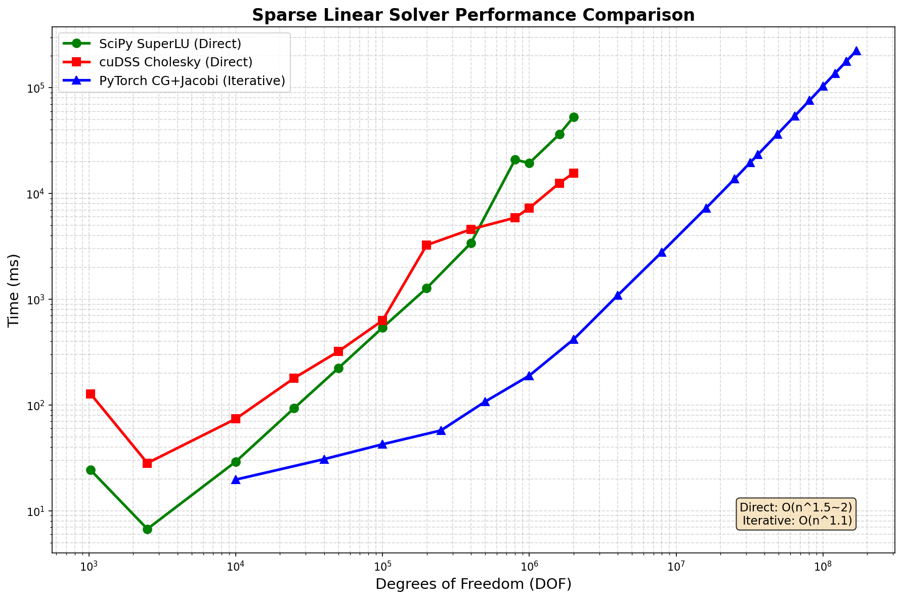
DOF	SciPy LU	cuDSS Cholesky	PyTorch CG+Jacobi	Notes	Winner
10K	24	128	20	All fast	PyTorch
100K	29	630	43		SciPy
1M	19,400	7,300	190		PyTorch 100x
2M	52,900	15,600	418		PyTorch 100x
16M	OOM	OOM	7,300		PyTorch only
81M	OOM	OOM	75,900		PyTorch only
169M	OOM	OOM	224,000		PyTorch only

Memory Usage¶

Memory Characteristics¶
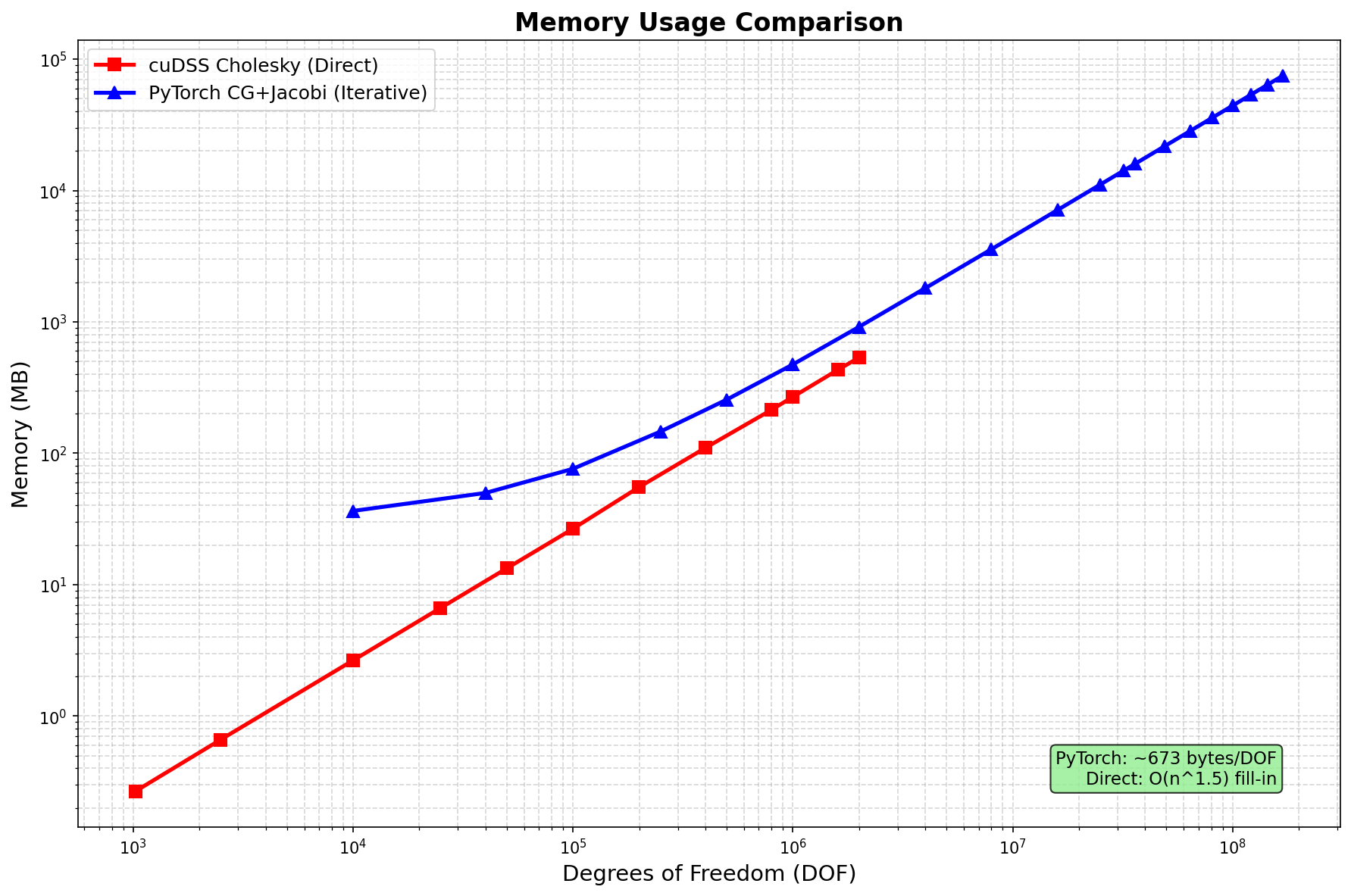
Method	Memory Scaling	Notes
SciPy LU	O(n^1.5) fill-in	CPU only, limited to ~2M DOF
cuDSS Cholesky	O(n^1.5) fill-in	GPU, limited to ~2M DOF
PyTorch CG+Jacobi	O(n) ~443 bytes/DOF	Scales to 169M+ DOF

Accuracy¶

Accuracy Comparison¶
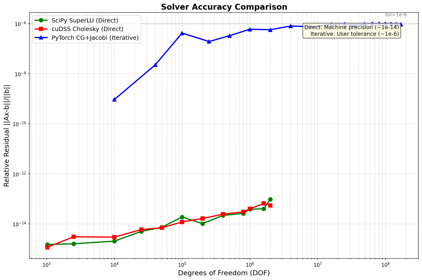
Method Type	Relative Residual	Notes
Direct (scipy, cudss)	~1e-14	Machine precision
Iterative (pytorch+cg)	~1e-6	User-configurable tolerance

Key Findings¶

The iterative solver reached 169M DOF with time scaling near O(n^1.1).
Direct solvers stopped near 2M DOF, bound by O(n^1.5) fill-in.
At 2M DOF, PyTorch CG with Jacobi was about 100x faster than the direct solvers.
PyTorch CG used ~443 bytes/DOF (the matrix and Krylov vectors; the bare CSR matrix is ~144 bytes/DOF).
Direct solvers reach machine precision; the iterative path reaches ~1e-6.

Distributed Solve (Multi-GPU)¶

On 3-4 NVIDIA H200 GPUs over NCCL, the distributed CG solve reached 400M DOF:

DOF	Time	Memory/GPU	GPUs
10K	0.1s	0.03 GB	4
100K	0.3s	0.05 GB	4
1M	0.9s	0.27 GB	4
10M	3.4s	2.35 GB	4
50M	15.2s	11.6 GB	4
100M	36.1s	23.3 GB	4
200M	119.8s	53.7 GB	3
300M	217.4s	80.5 GB	3
400M	330.9s	110.3 GB	3

Reading the table: 400M DOF fit on 3 H200s at 110 GB/GPU; going from 10M to 400M (40x the unknowns) cost ~100x the time, at ~275 bytes/DOF per GPU. At 100K DOF the GPU path took 0.3s against 7.4s on CPU.

# Run distributed solve with 3-4 GPUs
torchrun --standalone --nproc_per_node=3 examples/distributed/distributed_solve.py

Gradient Support¶

Every operation below is differentiable through PyTorch autograd. The solve and spectral ops use the adjoint method, so the backward pass costs O(1) autograd nodes rather than one per iteration.

SparseTensor Gradient Support

The adjoint column gives the backward rule. For a scalar loss \(L\), write \(g = \partial L/\partial x\) for the incoming gradient; \(A^{H}\) is the conjugate transpose.

Operation	CPU	CUDA	Adjoint / gradient	Notes
`solve()`	✓	✓	\(A^{H}\lambda = g,\ \partial L/\partial A = -\lambda x^{H}\)	Adjoint method, O(1) graph nodes
`eigsh()` / `eigs()`	✓	✓	\(\partial L/\partial A = \sum_i \bar g_{\lambda_i}\, v_i v_i^{H}\) (+ eigenvector term)	Adjoint method, O(1) graph nodes
`det()` / `logdet()`	✓	✓	\(\partial L/\partial A = \bar g\,\det(A)\,A^{-\top}\) (det); \(A^{-\top}\) (logdet)	Jacobi’s formula, reuses the LU factorization
`svd()`	✓	✓	\(\partial L/\partial A = U\,\mathrm{diag}(\bar g_\sigma)\,V^{H}\) (+ subspace term)	Power iteration, differentiable
`nonlinear_solve()`	✓	✓	\(J^{H}\lambda = g,\ \partial L/\partial\theta = -\lambda^{H}\,\partial r/\partial\theta\)	Adjoint at the fixed point, params only
`@ (A @ x, SpMV)`	✓	✓	\(\partial L/\partial x = A^{\top}g\)	Standard autograd
`@ (A @ B, SpSpM)`	✓	✓	\(\partial L/\partial A = G\,B^{\top}\) (on the sparse pattern)	Sparse gradients
`+`, `-`, `*`	✓	✓	Element-wise; gradient passes through the pattern	Element-wise ops
`T() (transpose)`	✓	✓	\(\partial L/\partial A = G^{\top}\)	View-like, gradients flow through
`norm()`, `sum()`, `mean()`	✓	✓	Standard reduction gradients	Standard autograd
`to_dense()`	✓	✓	Scatter dense grad back to the sparse pattern	Standard autograd

DSparseTensor Gradient Support

Operation	CPU	CUDA	Notes
`D @ x`	✓	✓	Distributed matvec, adjoint \(A^{\top}g\) (`VertexShard` halo exchange / `BatchShard` zero-comm)
`D.solve(b_dt)`	✓	✓	Distributed CG / BiCGStab / GMRES / FGMRES / MINRES; adjoint \(A^{H}\lambda=g\) (`VertexShard`)
`D.eigsh(k=)`	✓	✓	Distributed LOBPCG (`VertexShard`); per-rank batched eigsh (`BatchShard`)
`D.solve_batch_shard(b)`	✓	✓	Per-rank batched solve (`BatchShard`, zero comm)
`D.sum / .mean / .max / .min / .prod / .norm('fro' \| 1 \| inf)`	✓	✓	Cross-rank `all_reduce` over stored values
`D.is_symmetric / .is_hermitian / .is_positive_definite`	✓	✓	Cached `full_tensor()` + single-process check
`D.detect_matrix_type()`	✓	✓	Used by `solve(..., matrix_type='auto')`
`D.T() / .H()`	✓	✓	Allgather → transpose → repartition on same mesh
`D + s`, `D.abs()`, etc.	✓	✓	Local elementwise, same spec
`D.save / DSparseTensor.load`	✓	✓	Per-rank `partition_<rank>.safetensors` + `metadata.json`
`D.full_tensor()`	✓	✓	Allgather to a global `SparseTensor`
`D.det() / .lu() / .svd() / .condition_number()`	✓	✓	Falls back to `full_tensor()` + single-process compute; emits `ResourceWarning`
`D.nonlinear_solve()`	✓	✓	Distributed Newton-Krylov, adjoint \(J^{H}\lambda=g\)

Notes:

SparseTensor.solve() and eigsh() backprop via the adjoint method, so graph size is independent of iteration count.
DSparseTensor runs its algorithms (LOBPCG, CG, power iteration) on the sharded data; the core operations need no global gather.
For nonlinear_solve(), gradients flow to the parameters passed to residual_fn.

For backend-selection and performance guidance, see Performance Tips.

Citation¶

If you use torch-sla in your research, please cite our paper:

Paper: arXiv:2601.13994 - Differentiable Sparse Linear Algebra with Adjoint Solvers and Sparse Tensor Parallelism for PyTorch

@article{chi2026torchsla,
  title={torch-sla: Differentiable Sparse Linear Algebra with Adjoint Solvers and Sparse Tensor Parallelism for PyTorch},
  author={Chi, Mingyuan},
  journal={arXiv preprint arXiv:2601.13994},
  year={2026},
  url={https://arxiv.org/abs/2601.13994}
}