Operations
This is the per-operation reference. Operations are grouped by category;
each entry gives the signature, a one-line summary, a runnable example, an
input/output visualization, which class(es) it is available on, the API link,
and – where measured – a scaling plot. The two classes that carry these
operations are SparseTensor (single process, see
SparseTensor) and DSparseTensor (distributed, see
DSparseTensor).
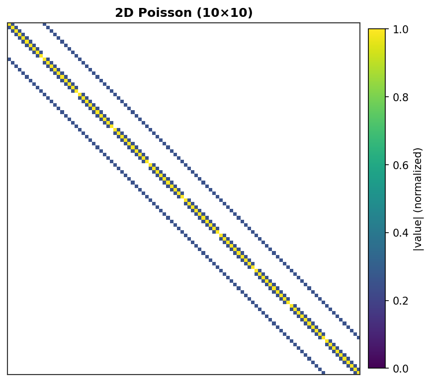
Throughout, A is a sparse matrix built from a 2D Poisson stencil; its
sparsity pattern looks like:
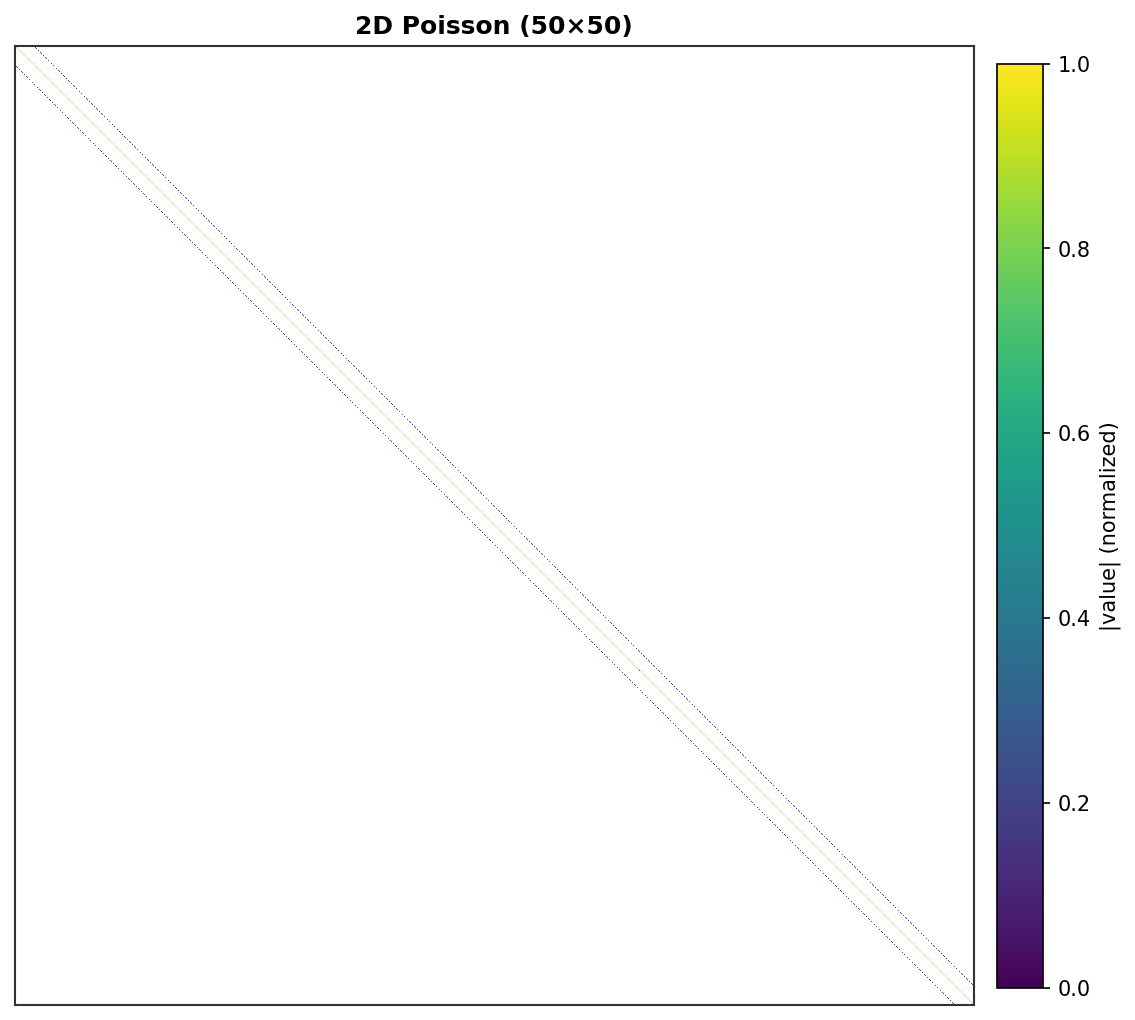
A.spy() for a 50×50 grid (2,500 DOF) – the banded 5-point stencil.
Scaling plots come from benchmarks/benchmark_all_ops_scaling.py (CPU = AMD
Ryzen 7 255; CUDA = RTX 4070 Ti SUPER). See Benchmarks for the full
methodology and the large-scale single-/multi-GPU numbers.
Linear solves
solve
A.solve(b, *, backend='auto', method='auto', **kwargs) -> x
Solve \(Ax = b\) for x, auto-selecting a direct (LU/Cholesky) or
iterative (CG/BiCGStab/GMRES) backend from the device and matrix type.
Example
import torch
from torch_sla import SparseTensor

dense = torch.tensor([[ 4.0, -1.0,  0.0],
                      [-1.0,  4.0, -1.0],
                      [ 0.0, -1.0,  4.0]], dtype=torch.float64)
A = SparseTensor.from_dense(dense)
b = torch.tensor([1.0, 2.0, 3.0], dtype=torch.float64)

x = A.solve(b)                      # auto: scipy+lu on CPU, cudss on GPU
x = A.solve(b, backend='pytorch', method='cg', preconditioner='jacobi')
Gradients flow through the solve via the adjoint method (O(1) graph nodes),
either by setting requires_grad on the values or via the functional
spsolve().
Input / output visualization
A.spy() shows the operator; the solve maps the right-hand side b to the
solution x = A⁻¹b. For an SPD system the CG residual decays as below.
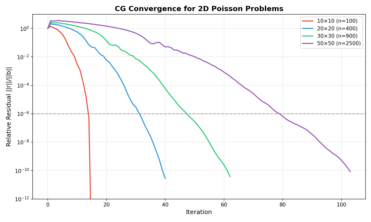
CG convergence for 2D Poisson systems of increasing size.
Available on SparseTensor,
DSparseTensor (see distributed solve).
API solve(), functional
spsolve().
Scaling

solve_batch
A.solve_batch(val_batch, b_batch, **kwargs) -> x_batch
Solve many systems that share one sparsity pattern but differ in values and/or right-hand sides, reusing a single symbolic factorization.
Example
from torch_sla import SparseTensor

A = SparseTensor(val, row, col, shape)

val_batch = torch.stack([val * (1.0 + 0.01 * t) for t in range(100)])  # [100, nnz]
b_batch   = torch.randn(100, n, dtype=torch.float64)                   # [100, n]

x_batch = A.solve_batch(val_batch, b_batch)                            # [100, n]
A leading batch dimension on the tensor itself (shape [B, n, n]) works the
same way through A.solve(b).
Input / output visualization Each batch element shares the A.spy()
pattern above; only the non-zero values change between elements.
Available on SparseTensor,
DSparseTensor (BatchShard layout).
API solve_batch().
Scaling

lu
A.lu(**kwargs) -> LUFactorization
Compute and cache an LU factorization so repeated solves with the same matrix skip refactorization – forward/back substitution only.
Example
from torch_sla import SparseTensor

A  = SparseTensor(val, row, col, shape)
lu = A.lu()                          # factorize once: O(nnz^1.5)

for t in range(100):                 # each solve is cheap: O(nnz)
    x_t = lu.solve(compute_rhs(t))
Input / output visualization A.spy() shows the operator; the factors
L and U retain its band plus fill-in.
Available on SparseTensor.
API lu(), LUFactorization.
Scaling

Nonlinear
nonlinear_solve
A.nonlinear_solve(residual_fn, u0, *params, method='newton', **kwargs) -> u
Solve \(F(u, \theta) = 0\) by Newton / Picard / Anderson iteration, with adjoint gradients w.r.t. the parameters (O(1) graph nodes, independent of the iteration count).
Example
import torch
from torch_sla import SparseTensor

A = SparseTensor(val, row, col, (n, n))

def residual(u, A, f):               # F(u) = A u + u^2 - f
    return A @ u + u**2 - f

f  = torch.randn(n, requires_grad=True)
u0 = torch.zeros(n)

u = A.nonlinear_solve(residual, u0, f, method='newton')
u.sum().backward()                   # f.grad via the adjoint method
Input / output visualization A.spy() shows the Jacobian’s sparsity
pattern, which Newton reuses each iteration.
Available on SparseTensor,
DSparseTensor (Shard(0) Newton, jac_diag_fn required).
API nonlinear_solve(), functional
nonlinear_solve().
Scaling

Eigen / spectral
eigsh / eigs
A.eigsh(k=6, which='LM', return_eigenvectors=True) -> (w, V)
Top-k eigenpairs of a symmetric/Hermitian matrix via LOBPCG/ARPACK
(eigsh()); eigs()
is the general (non-symmetric) counterpart. Eigenvalues are differentiable.
Example
from torch_sla import SparseTensor

A = SparseTensor(val, row, col, (n, n))

w, V = A.eigsh(k=6, which='LM')      # 6 largest, symmetric
w, V = A.eigsh(k=6, which='SM')      # 6 smallest
w, V = A.eigs(k=6)                   # general matrix

w = w.requires_grad_(); w.sum().backward()   # gradients flow to the values
Input / output visualization
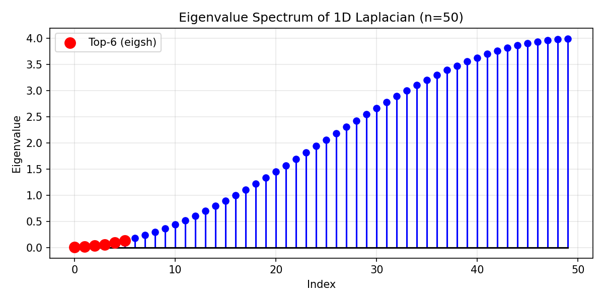
Eigenvalue spectrum of a 1D Laplacian (n=50); the 6 smallest computed by
eigsh(which='SM') are highlighted.
Available on SparseTensor,
DSparseTensor (see distributed eigsh).
Scaling

svd
A.svd(k=6) -> (U, S, Vt)
Truncated rank-k singular value decomposition, \(A \approx U_k \Sigma_k V_k^T\) – the best rank-k approximation in Frobenius norm. Differentiable.
Example
from torch_sla import SparseTensor

A = SparseTensor(val, row, col, (m, n))

U, S, Vt = A.svd(k=10)
A_approx = U @ torch.diag(S) @ Vt
error = (A.to_dense() - A_approx).norm() / A.norm('fro')
Input / output visualization
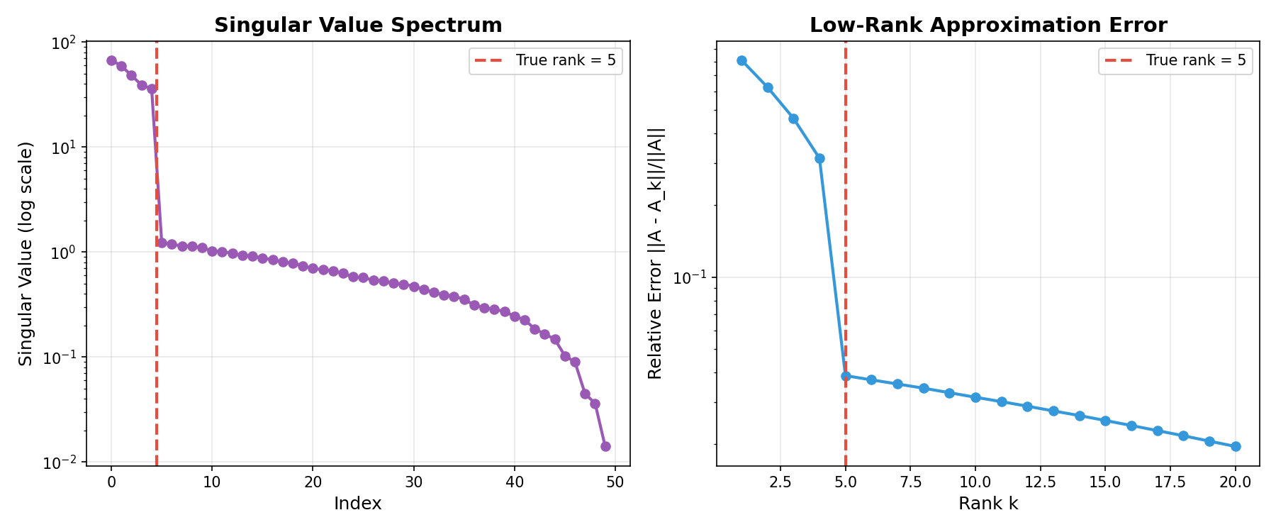
Left: singular-value spectrum (rapid decay past the true rank). Right: approximation error vs retained rank.
Available on SparseTensor.
API svd().
Scaling

Matrix–vector
matvec / @ (SpMV)
A @ x -> y (sparse matrix–vector or matrix–matrix product)
Sparse matrix–vector product \(y = Ax\). x may be a vector,
a stack of vectors, or another SparseTensor (sparse
matrix–matrix). The backbone of every iterative solver.
Example
from torch_sla import SparseTensor

A = SparseTensor(val, row, col, (n, n))
x = torch.randn(n, dtype=torch.float64)

y = A @ x                            # SpMV
Y = A @ torch.randn(n, 8)            # SpMM (8 right-hand sides)
Input / output visualization A.spy() shows which entries of x
contribute to each output: row i of y sums A[i, j] * x[j] over the
non-zeros in that row.
Available on SparseTensor,
DSparseTensor (halo-exchange SpMV, see
distributed matvec (halo-exchange SpMV)).
API __matmul__().
Scaling

Scalar / structural
det
A.det() -> torch.Tensor
Determinant via sparse LU (Jacobi’s-formula gradient through the adjoint
method). For CUDA tensors prefer A.cpu().det() – the GPU path densifies.
Example
from torch_sla import SparseTensor

dense = torch.tensor([[2.0, 1.0],
                      [1.0, 3.0]], dtype=torch.float64, requires_grad=True)
A = SparseTensor.from_dense(dense)
d = A.det()                          # 5.0
d.backward()                         # dense.grad = [[3, -1], [-1, 2]]
Input / output visualization A.spy() shows the operator; the
determinant is a scalar summary of it.
Available on SparseTensor,
DSparseTensor (gathers to one rank).
API det().
Scaling

logdet
A.logdet() -> torch.Tensor
Log-determinant – numerically stable where det would overflow/underflow.
Differentiable.
Example
from torch_sla import SparseTensor

A  = SparseTensor(val, row, col, (n, n))
ld = A.logdet()                      # log|det(A)|
Input / output visualization Same operator as det; see A.spy().
Available on SparseTensor,
DSparseTensor (gathers to one rank).
API logdet().
Scaling

norm
A.norm(ord='fro') -> torch.Tensor
Matrix norm: Frobenius (default), 1-norm, or 2-norm. Differentiable.
Example
from torch_sla import SparseTensor

A = SparseTensor(val, row, col, (n, n))
nf = A.norm('fro')
n1 = A.norm(1)
Input / output visualization A.spy() shows the entries the Frobenius
norm aggregates: \(\|A\|_F = \sqrt{\sum_{ij} a_{ij}^2}\).
Available on SparseTensor,
DSparseTensor.
API norm().
Scaling

condition_number
A.condition_number(ord=2) -> torch.Tensor
Condition number \(\kappa = \sigma_{\max}/\sigma_{\min}\); predicts how hard the system is to solve and how fast CG converges.
Example
from torch_sla import SparseTensor

A = SparseTensor(val, row, col, (n, n))
kappa = A.condition_number()
Input / output visualization A.spy() shows the operator; a wider band /
stronger anisotropy generally raises \(\kappa\).
Available on SparseTensor,
DSparseTensor (gathers to one rank).
API condition_number().
Scaling

is_symmetric / is_positive_definite
A.is_symmetric() -> bool · A.is_positive_definite() -> bool
Structural predicates used to pick a solver: a symmetric positive-definite
matrix admits Cholesky and CG; otherwise LU/BiCGStab.
is_hermitian() covers the complex case.
Example
from torch_sla import SparseTensor

A = SparseTensor.from_dense(dense)
A.is_symmetric()            # tensor(True)
A.is_positive_definite()    # tensor(True)
Input / output visualization A.spy() – symmetry shows as a pattern
mirrored across the diagonal.
Available on SparseTensor,
DSparseTensor.
API is_symmetric(),
is_positive_definite(),
is_hermitian().
Scaling Scaling plot coming soon (these are O(nnz) checks).
Graph
connected_components
A.connected_components() -> (labels, n_components)
Label the connected components of the matrix interpreted as a graph adjacency (FastSV: O(log N) parallel rounds, device-agnostic).
Example
from torch_sla import SparseTensor

A = SparseTensor(val, row, col, (n, n))
labels, n_components = A.connected_components()
Input / output visualization A.spy() reveals block structure: a
block-diagonal pattern means multiple components; a single dense band means
one.
Available on SparseTensor,
DSparseTensor (see distributed connected_components).
Scaling

Visualization
spy
A.spy(title=None, **kwargs) -> matplotlib.axes.Axes
Plot the sparsity pattern – one pixel per non-zero, intensity proportional to
|a_{ij}| – as a matplotlib figure. The input/output visualization used
throughout this page.
Example
from torch_sla import SparseTensor

A = SparseTensor(val, row, col, (n*n, n*n))
A.spy(title="2D Poisson (5-point stencil)")
Input / output visualization This is the visualization primitive:
Available on SparseTensor,
SparseTensorList.
API spy().
Scaling Not applicable (plotting utility).
Distributed
The operations below run on DSparseTensor; each mirrors a
single-process operation above and returns a rank-invariant result. See
DSparseTensor for the partitioning and halo-exchange model.
partition
DSparseTensor.partition(A, mesh, *, partition_method='simple', coords=None) -> D
Row-partition a global SparseTensor across a
DeviceMesh, computing the owned/halo layout once. The constructor for every
distributed operation.
Example
from torch.distributed.device_mesh import init_device_mesh
from torch_sla import SparseTensor, DSparseTensor

mesh = init_device_mesh("cuda", (world_size,))
A = SparseTensor(val, row, col, (n, n))
D = DSparseTensor.partition(A, mesh, partition_method="metis")
Input / output visualization A METIS partition groups rows so the
cross-partition halo (off-block non-zeros) is minimized; A.spy() on each
rank’s owned rows shows a near-block-diagonal slice plus a thin halo.
Available on DSparseTensor (classmethod). See also
partition_batch(),
from_global_distributed().
API partition(), functional
partition_graph_metis().
Scaling See the distributed scaling plots below.
distributed matvec (halo-exchange SpMV)
D @ x -> y
Distributed SpMV: each rank exchanges halo values with neighbors, then runs a local SpMV over its owned rows. The only intra-kernel communication in the distributed solvers.
Example
d = D.scatter(global_x)              # DTensor[Shard(0)]
y = (D @ d).full_tensor()            # gather result to global
Available on DSparseTensor. Mirrors
SparseTensor matvec.
API __matmul__().
Scaling

distributed solve
D.solve(b, **kwargs) -> x
Distributed Krylov solve of \(Ax = b\) in Shard(0) space: halo-exchange
SpMV plus all-reduce dot products, every vector kept rank-local. Sugar over
solve_distributed_shard; mirrors SparseTensor.solve.
Example
b = D.scatter(global_b)
x = D.solve(b)                       # distributed CG
x_global = x.full_tensor()
Available on DSparseTensor. Least-squares variants:
lsqr(), lsmr().
API solve().
Scaling

|

|
Strong scaling (speedup vs ranks) and weak scaling (time vs ranks, ideal flat). See Benchmarks for the multi-GPU run to 400M DOF.
distributed connected_components
D.connected_components() -> (labels, n_components)
Distributed FastSV: identical component labelling to the single-process version, computed across ranks with halo exchange.
Example
labels, n_components = D.connected_components() # rank's owned-slice + global count
Available on DSparseTensor. Mirrors
SparseTensor.connected_components.
Scaling Shares the single-process connected_components scaling; distributed strong/weak scaling under the distributed solve plots.
distributed eigsh
D.eigsh(k=6, which='LM', maxiter=200) -> (w, V)
Distributed LOBPCG for the top-k symmetric eigenpairs, with the same rank-invariant spectrum as the single-process solver.
Example
w, V = D.eigsh(k=6, which='LM') # same eigenvalues at every world size
Available on DSparseTensor. Mirrors
SparseTensor.eigsh.
API eigsh().
Scaling Shares the single-process eigsh scaling; distributed strong/weak scaling under distributed solve.